chenmoucheng.github.io

2-3 データ構造とアルゴリズム

Graph theory

The main reference here is Chapter 6 and 7 of the lecture notes on 『アルゴリズムとデータ構造』 by 松林昭先生, which we shall refer to as the lecture notes in this handout. We briefly review some of the most important definitions and facts that will be useful to us.

Definition. A set is a collection of distinct elements. We write x ∈ X if x is an element of the set X.

Definition. A function f from its domain X to its codomain Y associates exactly one element f(x) ∈ Y to each and every element x ∈ X. A function f from set X to set Y is often denoted as f: X→Y.

Definition. Given functions f: X→Y and g: Y→Z, the composition of f and g is a function g ⚬ f: X→Z defined by (g ⚬ f)(x) = g(f(x)) for all x ∈ X.

Definition. For a set X, there is a unique identity function 1: X→X on X that sends every x ∈ X to itself.

Definition. A function f: X→Y is surjective if for every y ∈ Y, there is at least one x ∈ X such that y = f(x). It is injective if f(x) = f(x’) implies that x = x’, or equivalently, x ≠ x’ implies f(x) ≠ f(x’).

Definition. A function f: X→Y is bijective if it is both surjective and injective, in which case it has an inverse g: Y→X such that g ⚬ f = 1 and f ⚬ g = 1.

Definition. A graph G is an unordered pair (V,E) of sets, where each v ∈ V is a vertex of G, and each e ∈ E, an edge of G. An edge connects two (not necessarily distinct) vertices.

Definition. A directed graph is graph G = (V,E) such that each edge e ∈ E is an ordered pair (u,v) for some u,v ∈ V, i.e., there are functions s,t: E→V such that for each edge (u,v) ∈ E, s(u,v) = u and t(u,v) = v.

In other words, we tend to think of an edge e ∈ E of a directed graph G = (V,E) as an arrow, pointing from its source s(e) to its target t(e).

Example (from the lecture notes). Let G = (V,E) for V = {a,b,c,d,e,f,g,h} and E = {(a,b), (a,c), (a,d), (b,d), (c,d), (d,e), (c,f), (f,g), (f,h), (g,h)}. In the lecture notes, there is a visualization of G as an undirected graph. You can use http://arborjs.org/halfviz to visualize G as a directed graph.

a -> b
a -> c
a -> d
b -> d
c -> d
d -> e
c -> f
f -> g
f -> h
g -> h

The visualization produced by http://arborjs.org/halfviz is interactive. For example, you can drag the vertices to make it look like the (undirected) graph in the lecture notes. As you can see, the edges in a directed graph are usually visualized using arrows, whereas in an undirected graph, lines.

So far we have been discussing simple graphs, which are graphs whose edges are sets; alternatively, G = (V,E) is a simple directed graph if the function (s,t): E→V×V is injective. We can generalize the notion to multigraphs, namely, graphs whose edges are multisets. For directed graphs, the function (s,t): E→V×V is no longer required to be injective, so there can be two edges e ≠ e’ but (s(e),t(e)) = (s(e’),t(e’)). In other words, the equality of edges of multigraphs is not predicated on the equality of their sources and targets, but rather on some other identities.

In contrast to the lecture notes, we are mainly interested in multigraphs. Unfortunately, http://arborjs.org/halfviz can only visualize simple graphs. You can try other (graph) visualization tools, such as Cytoscape.js, to see if you can visualize multigraphs.

Definition. A topological sort of a directed graph G = (V,E) is a linear ordering on V such that if there is an edge e ∈ E with s(e) = u and t(e) = v, then u ≤ v in the ordering.

Definition. A directed acyclic graph (DAG) is a directed graph that has a topological sort.

Remark. It follows immediately that a DAG does not have any directed cycles, so we could also define DAGs to be directed graphs without any directed cycles. These two definitions are equivalent.

Example. There exists a topological sort for the directed graph G in the above example, e.g., a ≤ b ≤ c ≤ d ≤ e ≤ f ≤ g ≤ h. Therefore, G is a DAG.

Exercise. Come up with a different topological sort for G and visualize it using http://arborjs.org/halfviz.

Terms and term DAGs

Graphs have numerous applications. In this experiment, we shall explore a particular application of DAGs to term unification.

Definition. Given a set V of variable symbols, a set C of constant symbols, and sets Fn of n-ary function symbols for each positive integer n, the set of (unsorted first-order) terms T is recursively defined to be the smallest set such that:

every variable symbol is a term: V ⊆ T;
every constant symbol is a term: C ⊆ T;
from every n terms t1,…,tn ∈ T and every n-ary function symbol f ∈ Fn, there is a term f(t1,…,tn) ∈ T.

Definition. The indegree of a vertex v ∈ V in a directed multigraph G = (V,E) is the number of edges going into v, i.e., |{ e ∈ E : t(e) = v }|. Similarly, the outdegree of v is the number of edges going out from v, i.e., |{ e ∈ E : s(e) = v }|.

Definition. A term DAG is a directed acyclic multigraph whose vertices are labeled with variable, constant, or function symbols, whose outgoing edges from any vertex are ordered, and where the outdegree of any vertex labeled with a function symbol f is equal to the arity of f.

Example. Let V = {x0,x1,x2}, C = {c}, F1 = {f}, F2 = {g}, F3 = {h}, F4 = F5 = … = ∅. Then T = {x0, x1, x2, c, f(x0), f(x1), f(x2), f(c), g(x0,x0), g(x0,x1), …, h(x0,x0,x0), h(x0,x0,x1), …, f(f(x0)), …, g(f(x0),h(x1,x2,f(c))), …}.

A web-based generator of random terms and term DAGs

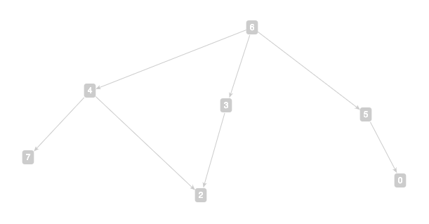
We provide term-graph, a web-based generator of random terms from T and their associated term DAGs. Let us take a closer look at the following example output and its visualization.

; h(g(c,x2),f(x2),f(x0))
; 6
-> 2
-> 7
-> 2
-> 0
-> 4
-> 3
-> 5

First, let us try to recover the missing vertex labeling in the term DAG, which is easy in such a toy example. For example, we observe that vertex 6 should be labeled with the function symbol h, as it is the only vertex with outdegree 3. Following the same line of reasoning, vertex 4 should be labeled with g. Now, when it comes to the other two outgoing paths 6→3→2 and 6→5→0, we know that both 3 and 5 should be labeled with f, but it is unclear whether we should label 2 with x0 or x2 (and vice versa for vertex 0). We have a similarly ambiguous situation when we try to label vertices 7 and 2 if we only look at the outgoing edges 4→7 and 4→2 from their common source vertex. In this example, fortunately, we have an additional piece of information that the subgraphs { 4→7, 4→2 } and { 3→2 } share a common vertex 2, which must correspond to the fact that the subterms g(c,x2) and f(x2) also share a common subterm x2. We can thus complete labeling all the vertices as follows.

Vertex	0	2	3	4	5	6	7
Symbol	`x0`	`x2`	`f`	`g`	`f`	`h`	`c`

We can now visualize this 7-vertex term DAG, again using http://arborjs.org/halfviz:

3"f" -> 2"x2"
4"g" -> 7"c"
4"g" -> 2"x2"
5"f" -> 0"x0"
6"h" -> 4"g"
6"h" -> 3"f"
6"h" -> 5"f"

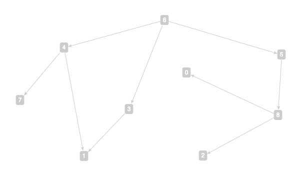
We conclude this (rather lengthy) example by two important observations. First, we note that term DAGs are by no means unique; sometimes a term can have two or more term DAGs. For example, you can verify that the following term DAG with 8 vertices also corresponds to the same term h(g(c,x2),f(x2),f(x0)):

3"f" -> 1"x2"
4"g" -> 7"c"
4"g" -> 2"x2"
5"f" -> 0"x0"
6"h" -> 4"g"
6"h" -> 3"f"
6"h" -> 5"f"

Last but not least, the ambiguity can be eliminated altogether if the outgoing edges from any vertex are indeed ordered, as the definition of term DAGs prescribes. However, this means that the (outgoing) edges would be a list, rather than a multiset.

Graph representations

Three representations of graphs are introduced in the lecture notes, namely, adjacency matrix, incidence matrix, and adjacency list.

Example. An adjacency matrix for the last term DAG is:

0 0 0 0 0 0 0
0 0 0 0 0 0 0
0 0 0 0 0 0 0
1 0 0 0 0 0 0
0 1 0 0 0 0 1
0 0 0 0 0 0 0
0 0 1 1 1 0 0
0 0 0 0 0 0 0

If we forget about the directions of the edges, then an incidence matrix for the same term DAG (when viewed as an undirected graph) is:

0 0 1 0 0 0
0 0 0 0 0 0
0 1 0 0 0 0
0 0 0 0 1 0
1 1 0 1 0 0
0 0 1 0 0 1
0 0 0 1 1 1
1 0 0 0 0 0

Since we are mainly interested in term DAGs, in which outgoing edges are ordered, we shall focus on adjacency list representations, e.g., for the same term DAG:

(0,[])
(1,[])
(2,[])
(3,[1])
(4,[7,2])
(5,[0])
(6,[4,3,5])
(7,[])

Basic data structures

To represent, e.g., graphs with a custom datatype in C, we typically use typedef to introduce our new datatype, along with a customary set of functional and managerial routines for manipulating instances of the new datatype. For example, we may need to test whether two instances of the new datatype are equal: the C programming language only supports equality on its primitive datatypes, so for more complicated, derived datatypes such as struct, we would need to implement our own equality tests. For datatypes whose storage size cannot be determined at compile time, we would also need dynamic memory management for creating, copying, as well as destroying the instances. Last but not least, we may also want to provide input/output functionalities for our new datatypes so that we can work and debug with them more easily.

Example.

typedef ... MyType;

int isEqMyType(const MyType *x, const MyType *y);   // x == y?
void copyMyType(MyType *x, const MyType *y);        // x <- y
const char *readMyType(MyType *x, const char* str); // x <- str
void showMyType(const MyType *x);                   // IO <- x
void freeMyType(MyType *x);                         // delete x

// example uses

MyType x, y;

readMyType(&x, input_string);
showMyType(&x); // should look the same as input_string
.
.
.
copyMyType(&y, &x);
assert(isEqMyType(&x, &y));
.
.
.
freeMyType(&x); 
freeMyType(&y); 

A more detailed example

Let us take a closer look at the following sample code. In this example, we have defined custom datatypes for vertices and edges, as well as lists of vertices and edges. Per our discussion above, we need dynamic memory management for lists but not for vertices and edges, as their storage sizes are known at compile time. With these datatypes, we can now define our Graph datatype using the adjacency list representation:

typedef struct {
    Vertex min,max;
    ListOfVertices *adj;
} Graph;

ListOfVertices *adj(const Graph *g, Vertex v)
{
    return g->adj + (v - g->min);
}

Here we assume that our vertices are numbered contiguously from min to max, and adj(&g, v) gives us the list of adjacent vertices of a vertex v connected by its outgoing edges in a graph g. We note that the two arguments are passed to adj differently: Graph g is passed by reference, whereas Vertex v, by value. In C programming, it is customary to pass instances of primitive datatypes by value and instances of more complicated, derived datatypes by reference, as is the case in this example.

Homework 1.

Implement the following five functions for handling lists of edges and give a few convincing test cases to show the correctness of your implementation.

int isEqListOfEdges(const ListOfEdges *es, const ListOfEdges *fs); // test if *es == *fs
void copyListOfEdges(ListOfEdges *es, const ListOfEdges *fs);      // copy fs to es
int isNullListOfEdges(const ListOfEdges *es);                      // test if *es == []
void showListOfEdges(const ListOfEdges *es);                       // print es to stdout
void freeListOfEdges(ListOfEdges *es);                             // free the memory used by es

/*
 * // Sample test vectors:
 * 
 * ListOfEdges es, fs;
 * 
 * readListOfEdges(&es, "2\n0 -> 1\n1 -> 2\n");
 * isNullListOfEdges(&es);    // 0
 * copyListOfEdges(&fs, &es);
 * isEqListOfEdges(&es, &fs); // 1
 * showListOfEdges(&fs);
 * // 2
 * // 0 -> 1
 * // 1 -> 2
 * freeListOfEdges(&es);
 * freeListOfEdges(&fs);
 */

Graph homomorphisms

Definition. A graph homomorphism φ from a graph G = (V,E) to G’ = (V’,E’) is a function from V to V’ that preserves the graph structure of G; that is, for any edge e = (s,t) of G, (φ(s),φ(t)) is an edge of G’. Furthermore, a bijective function φ from V to V’ is a graph isomorphism if both φ and its inverse are graph homomorphisms from G to G’, respectively. In this case, the two graphs G and G’ are isomorphic to each other.

Given a term, term-graph can also generate a random, isomorphic term DAG:

; h(g(c,x2),f(x2),f(x0))
; 6
-> 2
-> 7
-> 2
-> 0
-> 4
-> 3
-> 5

; 4
-> 7
-> 6
-> 5
-> 0
-> 2
-> 3
-> 2

It is easy to verify that these two graphs are isomorphic by the following vertex function φ:

v	0	2	3	4	5	6	7
φ(v)	0	2	6	7	5	4	3

Now we can apply φ to every vertex in the adjacency-list representation of the term DAG in our running example and arrive at the representation of the other, isomorphic term DAG:

(0,[])
(2,[])
(3,[])
(4,[7,6,5])
(5,[0])
(6,[2])
(7,[3,2])

Exercise. The term-graph can also generate a random term whose term DAG has at least certain number of vertices and edges. Run it a few times, generate a pair of larger, isomorphic term DAGs, and compute the isomorphism between them. Visualize both term DAGs using http://arborjs.org/halfviz and convince yourself that isomorphic graphs are indeed “the same”.

Topological sorts of a directed graph, revisited

We recall that a topological sort of a directed graph G = (V,E) is a linear ordering on V such that for every edge e ∈ E with s(e) = u and t(e) = v, u ≤ v in the ordering. Here we give a common way for computing a topological sort of a directed graph.

Algorithm (Kahn, 1962).

Input: Graph G = (V,E)
emptyListOfVertices(&L);
ListOfVertices S ← [ Vertex v | v ← vertices(&G) && indegree(&G, v) == 0 ];
while (!isNullListOfVertices(&S)) {
    Vertex u ← removeAtHeadListOfVertices(&S);
    appendListOfVertices(&L, u);
    foreach [ Vertex v | (u,v) ∈ E ] {
        G ← (V, E \ {(u,v)});
        if (indegree(&G, v) == 0) appendListOfVertices(&S, v);
    }
    G ← (V \ {u}, E);
}
return isNullListOfEdges(&E);
Output: ListOfVertices L (when E = ∅)

To prove the correctness of Kahn’s algorithm, we need to show that it terminates in a finite number of steps (for a finite input Graph G), and the output L represents a topological sort of the input Graph G when G is a DAG and when the algorithm terminates. First, we note that at each step of the while loop, the number of vertices of G monotonically decreases, so the algorithm must terminate after a finite number of steps. Next, for every edge (u,v) ∈ E, Kahn’s algorithm would never insert v before u into L because a vertex v needs to be in S before it can be inserted into L, which happens if and only if its indegree is or becomes 0, at which point all vertices u preceding v would have already been inserted into L. Finally, the algorithm terminates when there are no vertices of indegree 0 in G. At this time, G is either empty or not a DAG according to the following two lemmas, whose proofs we leave as an exercise.

Lemma. A (finite) DAG has at least one vertex of indegree 0.

Lemma. If we remove one or more vertices/edges from a DAG, then we would have another, possibly empty, DAG.

Homework 2.

Implement the following four functions and give a few convincing test cases to show the correctness of your implementation. You can use term-graph to check whether a list of vertices is a topological sort of a graph or not.

// The edges of a graph
void edges(ListOfEdges *es, const Graph *g);

// The indegree of a vertex of a graph
unsigned int indegree(const Graph *g, Vertex v);

// Test if a list of vertices is a topological sort of a graph
int isaTopSort(const ListOfVertices *vs, const Graph *g);

// A topological sort of a graph
int topSort(ListOfVertices *vs, const Graph *g);

/*
 * // Sample test vectors:
 * 
 * Graph g;
 * ListOfEdges es;
 * ListOfVertices vs;
 * 
 * readGraph(&g, "0\n8\n0\n0\n0\n3 6 7 8\n3 3 1 1\n1 6\n1 1\n2 0 0\n3 5 0 2\n");
 * edges(&es, &g);
 * showListOfEdges(&es);
 * // 13
 * // 3 -> 6
 * // 3 -> 7
 * // 3 -> 8
 * // 4 -> 3
 * // 4 -> 1
 * // 4 -> 1
 * // 5 -> 6
 * // 6 -> 1
 * // 7 -> 0
 * // 7 -> 0
 * // 8 -> 5
 * // 8 -> 0
 * // 8 -> 2
 * indegree(&g, 0);     // 3
 * indegree(&g, 4);     // 0
 * 
 * topSort(&vs, &g);
 * isaTopSort(&vs, &g); // 1
 * 
 * freeGraph(&g);
 * freeListOfEdges(&es);
 * freeListOfVertices(&vs);
 * /

Graph isomorphism algorithms

To this day, the worst-case complexity for solving the general graph isomorphism problem is not yet known, despite the existence of polynomial-time algorithms for solving many special cases. In particular, the isomorphism problem for term DAGs can be solved efficiently, and we are going to implement a simple algorithm that solves a subclass of it in this experiment.

Definition. A directed walk in a directed graph is a (possibly empty) sequence of edges (e_1, e_2, e_3, …) such that t(e_(i-1)) = s(e_i) and t(e_i) = s(e_(i+1)) whenever defined. A directed path is a directed walk going through distinct vertices, that is, when (s(e_1), t(e_1)=s(e_2), t(e_2)=s(e_3), t(e_3)=s(e_4), …) is a (possibly empty) sequence of distinct vertices.

Lemma. In a DAG, every directed walk is a directed path.

Definition. A root of a directed graph G = (V,E) is a vertex r ∈ V such that there is a directed path from r to every other vertex v ∈ V \ {r}.

Lemma. If a DAG has a root, then it has a unique root, in which case it is called a rooted DAG.

Lemma. Any term DAG associated with a term is rooted. Furthermore, the root of a term DAG is the least element under any of its topological sorts.

Definition. Recall that in a term DAG, the outgoing edges from any vertex are ordered. An access path of a vertex v in a rooted term DAG G = (V,E) is a (possibly empty) sequence of positive integers (p_1, p_2, p_3, …) such that there is a directed path (e_1, e_2, e_3, …) from the root of G to v, and for i = 1, 2, 3, …, p_i is the position of e_i among the outgoing edges of s(e_i).

Example. Let G be the following rooted term DAG.

; h(g(c,x2),f(x2),f(x0))
; 6
-> 2
-> 7
-> 2
-> 0
-> 4
-> 3
-> 5

An example rooted term DAG

Vertex	Access paths
0	(3,1)
2	(1,2),(2,1)
3	(2)
4	(1)
5	(3)
6	()
7	(1,1)

Exercise. Come up with a topological sort for G in the above example and verify that the root of G is indeed the least element in the topological sort that you come up with.

Lemma. In a rooted term DAG, distinct vertices cannot have identical sets of access paths.

Theorem. Let AP_v be the set of all access paths of a vertex v in a rooted term DAG. Then for all rooted term DAGs G = (V,E) and G’ = (V’,E’), G and G’ are isomorphic if and only if { AP_v : v ∈ V } = { AP_v’ : v’ ∈ V’ }.

Exercise. Let G’ be the following rooted term DAG. Find a graph isomorphism φ from G to G’.

; h(g(c,x2),f(x2),f(x0))
; 4
-> 0
-> 7
-> 5
-> 3
-> 2
-> 6
-> 2

Homework 3.

Implement the following two functions in the sample code and give a few convincing test cases to show the correctness of your implementation. Feel free to design and implement your custom, auxiliary datatypes to represent, e.g., access paths in order to achieve your goals.

// Test if a list of vertices represents an isomorphism between two rooted term DAGs
int isanIsomorphism(const ListOfVertices *phi, const Graph *g, const Graph *h);

// An isomorphism between two rooted term DAGs
int isomorphism(ListOfVertices *iso, const Graph *g, const Graph *h);

/*
 * // Sample test vectors:
 * 
 * Graph g, h;
 * ListOfVertices phi;
 * 
 * readGraph(&g, "1\n7\n0\n0\n1 2\n2 7 2\n1 1\n3 4 3 5\n0\n");
 * readGraph(&h, "1\n7\n0\n0\n0\n3 7 6 5\n1 1\n1 2\n2 3 2\n");
 * 
 * isomorphism(&phi, &g, &h);     // 1
 * showListOfVertices(&phi);      // 7 1 2 6 7 5 4 3
 * isanIsomorphism(&phi, &g, &h); // 1
 * 
 * freeGraph(&g);
 * freeGraph(&h);
 * freeListOfVertices(&phi);
 */

Term unification

Definition. Given a set C of constant symbols and sets Fn of n-ary function symbols for each positive integer n, we denote as T(X) the set of (unsorted first-order) terms on a set X of variable symbols. A (term) substitution φ: X→T(Y) is a function from X to T(Y), which uniquely determines a function from T(X) to T(Y) by replacing each occurence of every variable x ∈ X in a term t ∈ T(X) with φ(x) ∈ T(Y). By abuse of notation, this latter function from T(X) to T(Y) is also denoted by φ.

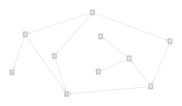
Example. Let X = {x0,x1,x2}, C = {c}, F1 = {f}, F2 = {g}, F3 = {h}, F4 = F5 = … = ∅. Let t = h(g(c,x2),f(x2),f(x0)) ∈ T(X) and φ: X→T(X) as follows.

x ∈ X	x0	x1	x2
φ(x) ∈ T(X)	g(x0,x2)	x1	x1

Then φ(t) = h(g(c,x1),f(x1),f(g(x0,x2))), and (φ ⚬ φ)(t) := φ(φ(t)) = h(g(c,x1),f(x1),f(g(g(x0,x2),x1))).

A term DAG for φ(t)

A term DAG for (φ ⚬ φ)(t) = φ(φ(t))

Definition. A substitution φ: X→T(Y) is said to unify a set of term equations in X, { s_i = t_i : i ∈ I }, if ∀ i ∈ I, φ(s_i) = φ(t_i).

Theorem. If a set E of term equations has a unifier, then it has a most general unifier φ in the sense that for any unifier φ’ of E, there is a unique substitution ψ such that φ’ = ψ ⚬ φ.

Definition. A rooted term DAG G is a tree if and only if there is a unique access path from the root to every other vertex of G. In contrast, G is fully collapsed if and only if no two rooted subgraphs of G are isomorphic.

Now we are ready to give a high-level description of a recursive descent algorithm for computing the most general unifier of two terms s and t. We start by computing G_s and G_t, the fully collapsed rooted term DAGs for s and t, respectively. Then we apply the following recursive algorithm to r_s and r_t, the roots of G_s and G_t, respectively, and the result will be the most general unifier (if exists) of s and t.

Algorithm.

unify(s,t)
{
  if (s == t) {
    φ = the identity substitution 1;
  }
  else if (s is a variable symbol x && x does not appear in t) {
    φ = the substitution that sends x to t and fixes all other variables;
  }
  else if (t is a variable symbol x && x does not appear in s) {
    φ = the substitution that sends x to s and fixes all other variables;
  }
  else if (s == f(s_1, ..., s_n) && t == f(t_1, ..., t_n)) {
    // f is an n-ary function symbol
    for (i = 1; i <= n; i++) {
      φ_i = unify(s_i, t_i);
    }
    φ = φ_n ⚬ ... ⚬ φ_1;
  }
  else return FAIL;

  G_s = φ(G_s);
  G_t = φ(G_t);
  return φ;
}